
The text bellow has been rejected by: Nature, Science, Physics Reports, Reviews of Modern Physics, Physical Review Letters and arXiv without even reaching a referee stage 🙂
Please, let me know if you have an idea how to extend the list above.
Although, quantum mechanics is the same for microscopic and macroscopic objects, there is a perception that the later do not exhibit basic quantum properties like superposition or interference. Historically this view has been encapsulated in a story called Schrödinger’s cat paradox, where a cat is, in full agreement with the rules of quantum mechanics, prepared in a superposition of two states: dead and alive. The paradoxical part is that no one has ever seen such a situation in the real world where large object would be simultaneously dead and alive or in two distinct places at the same time.
Here I show that there is no difference, in principle, between large and tiny objects. In fact, quantum features absent for large objects can be easily suppressed for microscopic objects as well. Moreover, I demonstrate that in transition from micro- to macro-world there is no need for any arbitrary quantum-classical border or any assistance from an external environment to resolve the paradox.
Introduction
Quantum mechanics (QM) is being developed for over 80 years, but one cannot say that the theory has matured by now. To the contrary, fundamental issues within quantum mechanics are still debated. What is the meaning of wave function – does it represent only ensembles or also individual objects? How to deal with the measurement process – should the measuring apparatus be classical or quantum? Is the measurement process part of quantum mechanics at all?
Even if the correct resolutions of those problems can be found in the literature, none of them are uniformly accepted by physicists.
In such circumstances, an argument that hopes to settle one of the great issues in QM in an easily reproducible way may be of interest to the scientific community.
In the following, a superposition of two spatial states will be considered rather than the dead and alive states. This choice comes with no harm to the generality of the solution, still it is simpler to quantify position of an object than vitality of an animal.
The well known Young double-slit experiment is one of the core examples of intrinsic workings of QM. It is also suitable for illustrating the resolution of the Schrödinger’s cat paradox.
A single photon “paradox”
Two slits, that are placed in the way of photons, produce an illumination pattern on a screen or a detector array. See Fig.1. Each photon passing the slits will leave a single dot on the screen. The relative position of slits and the screen affect the pattern.
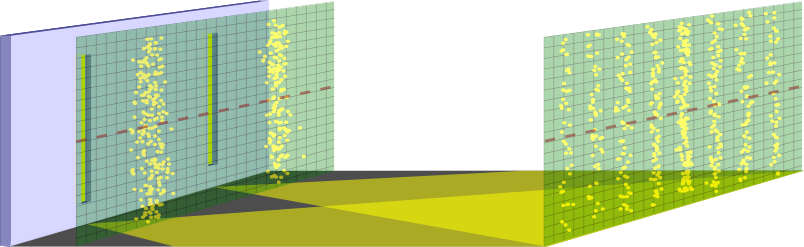
Fig. 1.Young experiment setup with screen either close to the slits (t = 0.02) or far away from them (t = 2.2).
In particular, if the screen is close to the slits, two fringes will appear. The fringes are just projected images of the two slits, Fig.1. For each yellow point on the screen there is no doubt where the photon, that produced it, came from. The left fringe corresponds to the left slit, the right fringe to the right slit. If one blocks, say, the right slit, the left fringe will stay the same.
If the screen is far enough from the slits, many interference fringes appear and there is no way to determine the origin of any photon that has reached the screen. In fact, the presence of the interference fringes is a manifestation of that indeterminism. Any successful attempt to track the photons back to a slit would destroy the interference pattern. In both cases, screen close to the slits and far from them, the quantum state of the photon is a superposition of two possibilities: photon originated from the left slit and photon originated from the right slit. However, in the first case, one can tell from which slit did the photon emerge because the two superposing states are spatially separated, Fig.2 a).
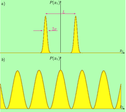
Fig. 2. Probability density along the dashed line in the screen of Fig.1 with screen a) close to the slits (t = 0.02) or b) far away from them (t = 2.2).
Therefore, if one formulated a single photon paradox in this fashion: Why don’t we see a superposition of a photon when the screen is close to the slits? After all, it has been prepared in the superposition of the left slit + right slit states. the answer is clear. We don’t see any superposition with a single photon because it leaves only one mark, in the left or the right fringe. It could happen that the mark will be left in the region between the fringes. In such case one may not be able to determine which slit the photon has passed through. It is, how- ever, less and less probable with the increasing L/σ ratio. We could infer about the superposition by repeating the single photon experiment many times and recording the two fringes that indicate the superposition (or mixture of states).
If, in the single photon paradox, we replace the word ”superposition” with ”interference” then the answer is that the two superposing states are spatially separated and there is no interference possible. One can firmly tell which slit the photon has originated from. There are only left-slit-photons and right-slit-photons and each mark on the screen belongs to one of the two. For the far away screen, we still will not see any superposition with just one photon, because a single spot on the screen does not reveal any. However, after many repetitions of the same experiment, we can learn that the interference pattern emerges, Fig.3 b). To prove that, one can block one of the slits and the interference fringes will not form.
To summarize, a single photon behaves similar to a hypothetical Schrödinger’s cat when the screen is close to the slits. Despite being described by a superposition of left-slit plus right-slit states it cannot show any signs of the superposition or interference. If experiment is repeated many times, only left-slit or right-slit photons are detected. Likewise, only alive or dead cat can be seen in the paradox. The similarity is explained in the next section.
Schrödinger’s cat state
There are many possible and equivalent versions of the Schrödinger’s cat state. The essential part is that they involve superposition of an object consisting of large number of quantum elements.
Within the setup of the Young experiment, one can produce such a state, too. It corresponds to the following arrangement: N photons passing through the left slit and no photons passing through the right slit plus no photons passing through the left slit and N photons passing through the right slit. N is of order of Avogadro number i.e. about 1024.
Symbolically, the Schrödinger’s cat state can be denoted as
(1) 
where the left slot in the |…, …〉 ket stands for the left slit, later represented by a Gaussian centered in position −L/2, and the right slot for the right slit, later represented by a Gaussian centered in position L/2.
Conveniently, the state of a single photon considered in previous section has the same form but with N = 1.
Fringes appearing on the screen are completely determined by the state from Eq.(1). For N = 1 the probability density across the dashed brown line in plane of the screen in the Fig.1 has this form:
(2) 
where x1 is a position variable along that line, L is the slits separation,σ≪L corresponds to the width of the slits and parameter t describes distance of the screen from the plane of the slits. The Eq.(2) has an interesting structure, it is a sum of three components. First two components describe the two fringes that are projections of the slits, the third one is an interference term. For example, if the distance of the screen from the slits is small i.e. t≪σ, the interference term is suppressed by the exponent with L2≫ σ2 and only two fringes remain, Fig.2 a).
On the other hand, for far away screen i.e. t/σ≫L the interference term dominates, Fig.2 b).
When more than one photon state is considered, there is a slight complication with the picture. Each photon brings an extra dimension to the probability density. For N photons the Eq.(2) turns into
(3) 
where index j counts the photons. Despite the multidimensional character, the probability density has a similar structure to that of one-photon state: the first two terms in the sum correspond to the projection of the slits on the N-dimensional space span by x1, …, xN variables and the third term is an interference component. The multidimensional analysis of the Eq.(3), even for N ∼ 1024, is quite straightforward. The interference term is suppressed even faster than before due to the N factor in the exponent with L2. The two remaining multivariate Gaussians have radius√(σ2 + (t/σ)2) and centers at (x1 = −L/2, …, xN = −L/2) i (x1 = L/2, …, xN = L/2).
The geometric distance of the centers is L√N, which is a large number as compared to the radius for moderate values of t. Thus, the two components of the probability density are spatially separated due to the large number of photons comprised by the Schrödinger’s cat.
Another way of inspecting the probability density is to use its one-dimensional cross section
x/√N = x1 = … = xN along the line that connects the centers of the two multivariate Gaussians i.e. passing through points (x1 = −L/2, …, xN = −L/2) i (x1 = L/2, …, xN = L/2)
(4) 
The cross section shows that large N will supress the interference term and expand the distance of the remaining Gaussians by factor √N. Again, the two Gaussians will be spatially separated for moderate values of t. That, in turn, implies that even if the screen is far away from the slits there will be neither interference pattern nor any ambiguity as to where each cat came from, the left or the right slit. All the events that are somewhere in the middle of the two Gaussians are highly improbable.
Conclusions
By varying N in (2) i (3) from 1 to 1024 one can explore the transition from micro- to macro-world all in terms of the Young experiment. The spatial separation of the multivariate Gaussians in the probability density goes from L to 1012L. Therefore, in macroscopic case, an experiment with one cat will necessarily reveal the cat passing through the left or the right slit.
The transition is smooth an has no place for the quantum-classical border. In fact, the end result for the Schrödinger’s cat state is very similar to the single photon state with the screen close to the slits. The lack of superposition and interference has exactly the same explanation in the two cases. One can say, that the Schrödinger’s cat state is as mysterious as a single photon state with the screen close to the slits.
Schrödinger’s cat versus photon (pdf)
Zbigniew Karkuszewski, December 19-th 2013
下面的文本被《自然》、《科学》、《物理报告》、《现代物理评论》、《物理评论快报》和arXiv拒绝,甚至没有进入审稿阶段 🙂
请告诉我是否有任何想法可以扩展上面的列表。
尽管微观和宏观物体的量子力学是相同的,但有一种看法认为后者不表现出像叠加或干涉这样的基本量子特性。从历史上看,这种观点已经被包含在一个叫做薛定谔猫悖论的故事中,其中一只猫按照量子力学的规则准备在两种状态中的一种:死和活。悖论的部分在于在现实世界中从未见过这样的情况,即大对象同时死和活,或在同一时刻处于两个不同的地方。
在这里,我展示了在原则上,大对象和微小对象之间没有区别。事实上,对于微小对象来说,对大对象不可见的量子特性也可以轻松被抑制。此外,我证明在从微观到宏观世界的过渡中,没有必要设定任何任意的量子-经典边界或依赖外部环境来解决这个悖论。
简介
量子力学(QM)发展已有80多年的历史,但不能说该理论目前已经成熟。相反,量子力学内部仍在讨论基本问题。波函数的含义是仅表示集合还是同时表示个体对象?如何处理测量过程 – 测量仪器应该是经典的还是量子的?测量过程是否根本属于量子力学?
即使这些问题的正确解决方案可以在文献中找到,但其中没有一个被物理学家们普遍接受。
在这种情况下,一个试图通过一种容易再现的方式解决QM中的重大问题的论点可能对科学界很有兴趣。
在接下来的内容中,将考虑两个空间状态的叠加,而不是死和活的状态。这个选择对解决方案的一般性没有伤害,但量化一个物体的位置比量化一个动物的生命力更简单。
众所周知的杨氏双缝实验是量子力学内在工作原理的核心例子之一。它也适合用来说明薛定谔猫悖论的解决方法。
单光子“悖论”
放置在光子路径中的两个狭缝在屏幕或探测器阵列上产生照明图案。见图1。穿过狭缝的每个光子都会在屏幕上留下一个单独的点。狭缝和屏幕的相对位置会影响图案。
图1. 靠近狭缝的屏幕(t = 0.02)或远离狭缝的Young实验设置(t = 2.2)。
特别是,如果屏幕离狭缝很近,将出现两个明显的条纹。这些条纹只是两个狭缝的投影图像,如图1所示。对于屏幕上的每个黄点,我们可以确定产生它的光子来自哪个狭缝。左侧的条纹对应于左侧的狭缝,右侧的条纹对应于右侧的狭缝。如果封住右侧的狭缝,左侧的条纹将保持不变。
如果屏幕离狭缝足够远,将出现许多干涉条纹,没有办法确定到达屏幕的任何光子的起源。事实上,干涉条纹的存在表明了这种不确定性。任何成功追踪光子返回到一个狭缝的尝试都会破坏干涉图案。在两种情况下,即屏幕靠近狭缝和远离狭缝时,光子的量子状态都是来自左侧狭缝的光子和来自右侧狭缝的光子的叠加状态。然而,在第一种情况下,我们可以根据光子的空间位置确定它是从哪个狭缝出来的,如图2a所示。
Fig. 2. 在图1的屏幕上沿虚线的概率密度,其中 a) 屏幕靠近狭缝(t = 0.02),或者 b) 屏幕远离狭缝(t = 2.2)。
因此,如果以这种方式表达了单光子悖论:当屏幕靠近狭缝时,我们为什么看不到一个光子的叠加态呢?毕竟,它已经被准备成了左狭缝+右狭缝状态的叠加态。答案很明确。我们在单个光子时看不到任何叠加态,因为它只留下一个标记,要么在左边要么在右边的波峰。它可能会发生在波峰之间的区域留下标记。在这种情况下,我们可能无法确定光子穿过了哪个狭缝。然而,随着L/σ比例的增加,这种可能性越来越小。通过多次重复单光子实验并记录指示叠加态(或状态混合)的两个波峰,我们可以推断出叠加态。
如果在单光子悖论中,我们用“干涉”代替“叠加”这个词,那么答案是两个叠加态是空间分离的,没有可能发生干涉。人们可以清楚地知道光子来自哪个狭缝。只有左狭缝光子和右狭缝光子,屏幕上的每个标记都属于其中之一。对于远处的屏幕,我们仍然看不到任何叠加态,因为屏幕上的一个单独点并没有显示任何叠加态。然而,经过多次重复相同实验后,我们可以了解到干涉图案的出现,如图3 b)所示。要证明这一点,可以堵住其中一个狭缝,干涉波峰就不会形成。
总之,当屏幕靠近狭缝时,单个光子的行为类似于一个假设中的薛定谔猫。尽管被描述为左狭缝加上右狭缝状态的叠加态,但它无法显示任何叠加态或干涉的迹象。如果实验多次重复,只检测到左狭缝或右狭缝的光子。同样,在悖论中只能看到活着或死去的猫。这种相似性在下一节中解释。
薛定谔猫态
薛定谔猫态有许多可能且等效的版本。其中关键部分是它们涉及对由大量量子元素组成的物体的叠加态。
在Young实验的设置中,我们也可以产生这样一个状态。它对应于以下安排:通过左缝的N个光子,右缝没有光子,加上左缝没有光子,右缝通过N个光子。这里N的数量级是阿伏伽德罗常数,即约为1024.。
符号上,薛定谔猫态可以表示为
(1)
其中|…, …〉ket 中的左槽代表左缝,后来用位置为 −L/2 处的高斯表示,右槽代表右缝,后来用位置为 L/2 处的高斯表示。
方便起见,在前一节中考虑的单个光子的状态具有相同的形式,但 N = 1。
出现在屏幕上的条纹完全由方程(1)中的状态确定。对于 N = 1,在图1的屏幕平面上,沿着虚线棕线的概率密度具有以下形式:
(2)
其中,x1 是沿该线的位置变量,L 是缝的间距,σ≪L 对应于缝的宽度,参数 t 描述屏幕与缝平面的距离。方程(2) 具有有趣的结构,它是三个分量的和。前两个分量描述了两个槽的投影,第三个是一个干涉项。例如,如果屏幕距缝很近,即 t≪σ,则通过 L2≫ σ2 的指数抑制了干涉项,只剩下两个条纹,图2a)。
另一方面,对于远离的屏幕,即 t/σ≫L,干涉项占主导地位,图2b)。
当考虑多个光子状态时,图片会稍微复杂化。每个光子都为概率密度带来了额外的维度。对于 N 个光子,方程 (2) 变成了:
(3)
其中索引 j 计数光子。尽管具有多维性,概率密度的结构与单光子状态相似:求和中的前两项对应于在由 x1, …, xN 变量张成的 N 维空间上的缝的投影,第三项是一个干涉分量。即使对于 N ∼ 1024,方程(3)的多维分析也是相当简单的。由于指数中的 N 因子,干涉项的抑制甚至比以前更快,剩下的两个多变量高斯分布的半径为√(σ2 + (t/σ)2),并且在以下位置:(x1 = −L/2, …, xN = −L/2) i (x1 = L/2, …, xN = L/2).
中心的几何距离为 L√N,与 t 的适度值相比,这是一个大的数字。因此,由于包含在薛定谔猫中的光子数量众多,概率密度的两个组分在空间上是分开的。
检查概率密度的另一种方法是使用其沿着连接两个多变量高斯分布中心的线的一维横截面x/√N = x1 = … = xN,即通过以下点:(x1 = −L/2, …, xN = −L/2) i (x1 = L/2, …, xN = L/2)
(4)
横截面显示,大 N 将抑制干涉项,并通过√N因子扩展剩余高斯分布的距离。再次,对于适度的 t 值,这两个高斯分布将在空间上分开。这反过来意味着,即使屏幕远离狭缝,也既不会有干涉图案,也不会有任何关于每只猫来自左狭缝还是右狭缝的歧义。两个高斯分布之间的所有事件都是极不可能的。
结论
通过在 (2) 和 (3) 中变化 N 从 1 变到 1024,可以在 Young 实验的术语中全面探讨从微观到宏观的过渡。概率密度中多元高斯分布的空间分离从 L 变到 1012L。因此,在宏观情况下,进行一次猫的实验将必然揭示猫通过左侧或右侧的狭缝。
过渡是平稳的,没有量子-经典边界的地方。事实上,对于薛定谔的猫态,最终结果与屏幕靠近狭缝的单光子态非常相似。在这两种情况下,缺乏叠加和干涉的解释完全相同。可以说,薛定谔的猫态和屏幕靠近狭缝的单光子态一样神秘。
Zbigniew Karkuszewski, 2013 年 12 月 19 日